
Data Augmentation Automation
Introduction
During the last few years, Deep Learning models have made incredible progress in classification problems thanks to the advances in deep network architectures, computational power and access to huge amounts of big data where they excel.
One of the most prominently used techiques for improving state of the are Deep Image Classifiers is Data augmentation. In this post, we test different ways of applying this technique and compare the results obtained to provide empirical evidence that these methods indeed improve the classification power of Deep Learning models.
The experiments will show that using different kinds of data augmentation improves the generalizing capabilities of the models on both a subset of the Fashion-MNIST dataset and of the full dataset. We will focus on obtaining good results where most of the classic models fail, namely on the differentiation of two specific classes of the dataset (shirt, tshirt/top).
Furthermore, we propose a way of speeding up the fine-tuning of augmentation parameters by using transfer learning by training a model using the original data and incrementally adding different augmentations to obtain the most robust model that generalizes the best. The paper and supplement code is available at link
Dataset
In this paper we will be using data augmentation techniques to show that they indeed improve the accuracy of a CNN model on the Fashion-MNIST dataset. Fashion-MNIST is a dataset of article images—consisting of a training set of 60,000 examples and a test set of 10,000 examples. Each example is a 28x28 grayscale image, associated with a label from 10 classes. The dataset has no null values and is ready-usable. Each pixel has a value from 0 to 255 representing the color of the pixel. The only preprocessing that was needed was standardizing the values which we do with min-max feature scaling
\[\frac{X-X_{min}}{X_{max}-X_{min}}\]Analyzing the dataset, we concluded that most of the classic ML models (SVMs, Random Forests, KNNs), as well as simple DNNs achieve an accuracy of 85%-90% and in all of them the main struggle was differentiating between two out of the ten classes, namely the shirt and t-shirt classes. In order to better evaluate the effects of the data augmentation we used two partitions of the dataset: one containing only samples of the two previously mentioned classes and one containing all of them. By doing this, we were able to speed up the processes of validating different augmentation techniques and combinations of the same, and test whether when applied to the whole dataset they obtained better results, i.e. whether the same augmentations could be used on different images to achieve a higher accuracy.
| Classifier | Accuracy |
|---|---|
| KNN | 0.840 |
| SVC | 0.861 |
| RF | 0.856 |
| CNN | 0.913 |
Methodology
In this section, we will explain the methodology followed to conduct the experiments, the type of NN architecture used and the types of data augmentation techniques that we tested.
Architecture
Since the main focus of this paper is the data augmentation part, we decided to keep the network architecture as simple as possible for maximum reproducibility.
The network consists of two convoluted blocks followed by a dense, fully connected layer. The building blocks are two pairs of convolutional layers followed by a batch normalization layer to stabilize the learning process and reduce the number of training epochs. Each building block ends with an average pooling layer to reduce the number of parameters to learn and prevent gross over-fitting. To test the network, we decided to preserve its simplicity by avoiding using momentums, decays, paddings. We used the Cross Entropy metric to measure the models and used the RMSProp Optimizer.
Also, a stable learning rate scheduler was used to decrease the learning rate by a factor of \(e^{-0.1}\) once every 10 epochs. This ensured the network has a chance of escaping local minima during the late stages of training.
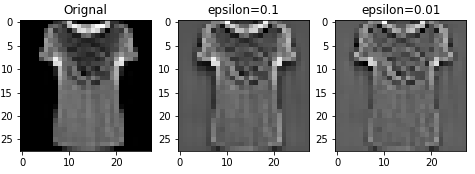
ZCA Whitening
Whitening is a linear transformation that transforms a vector of random variables with a known covariance matrix into a set of new variables whose covariance matrix is the identity matrix, meaning that they are uncorrelated and have variance 1. We are training on images, so the raw input is redundant, since intuitively, adjacent pixel values are highly correlated. What we want to solve with whitening is to ensure our network sees feature that are less correlated with each other and they all have the same variance.
More formally, a general whitening transforms a random vector \(x\) into a random vector \(z\) using a whitening matrix \(W\) while the original covariance matrix \(cov(x)=\Sigma\) becomes the identity matrix \(cov(z)=I\). ZCA whitening is based on the eigen-vectors \(U\) and eigen-values \(\Lambda\) of the covariance matrix which can be decomposed as: \(\Sigma = U\Lambda U^T\). Now, the whitening matrix can be written as:
\[W^{ZCA}=U\Lambda^{-\frac{1}{2}}U^T\]A parameterized formula has been used in Pal et al. where \(\epsilon\) is the whitening coefficient and \(S\) is the singular values of the initial set of images: \(W^{ZCA}=Udiag\left(\frac{1}{\sqrt{diag(S)+\epsilon}}\right)U^T\)
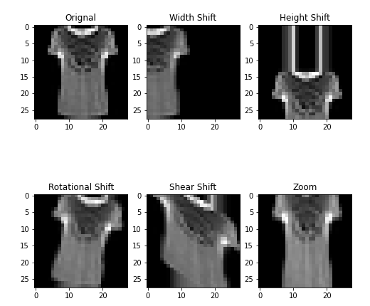
Positional Augmentation
Positional augmentation is the most common technique for adding variation to image datasets and it is also the simplest and most intuitive ones. This method doesn’t change the values of single pixels but rather applies a “shift” of the whole image relative to some base axis. The transformations that can be applied can be divided into three main subgroups:
- Axis Shifting: width, height and depth shifting (zoom)
- Rotational Shifting: Rotation and Shear
- Flips: Horizontal and Vertical
Data Augmentation Automation (DAA)
During the past few year significant improvements have been made in the process of automatic hyper-parameter finding. For finding the best combination of label-invariant augmentation hyper-parameters we propose a procedure comprising of 2 steps.
- As a first step we train our network without any data augmentation i.e. just the raw training data. This gives a starting point for tuning the hyper-parameters.
- Next, we develop a sequence of combinations of hyper-parameters to choose from and augment the training data. During this step one of two scenarios may occur. In the first case, the model performs worse and we obtain worse results than the base model in which case we fallback to the previous model weights and try another option of parameters (This is the option we want to avoid). In the second case, our model performs better and we keep the new model weights. Additionally, to prevent overfitting, we reduce the number of training steps by a constant factor for the next iteration and continue until there are no combinations left. The demo code is available here.
Experiments
Like we discussed in the introduction and , we carried out two types of experiments: firstly testing the augmentation techniques on the hard subset of shirts and t-shirts and secondly applying the best options that we obtained during the first trials on the full Fashion-MNIST dataset to determine whether the overall generalizing capabilities of the networks improved.
| Width Shift | Height Shift | Zoom | Rotation | ZCA | Accuracy |
|---|---|---|---|---|---|
| 0.913 | |||||
| 0.1 | 0.1 | 0.919 | |||
| 0.12 | 5 | 0.928 | |||
| 0.12 | 10 | 0.01 | 0.913 | ||
| 0.1 | 0.1 | 0.2 | 0.920 | ||
| 0.12 | 0.12 | 0.1 | 0.925 |
From the results, we can see that some combinations of augmentation techniques perform fairly better relative to the no augmentation CNN result. Another thing that we noticed during the experimentation phase is the fact that a combination between positional augmentations and whitening in the same trial yielded worse results than when we applied them distinctly. Moreover, positional augmentations complement each other very well and combining them yields the best models.
Using the methodology described in 3.4. we were able to pick a subset of combinations that worked best for the MNIST subset and tried to use them for training the network on the entire dataset. The subset of combinations obtained improved the generalization ability of the network proposed in 3.1. by ~1-2\% after averaging multiple trials. The best accuracy that was achieved was 95.04\% which is an improvement of the baseline model with no augmentation by about 1.56\% which is in line with the improvements obtained on the smaller subset.
Conclusion and Further Work
What this paper shows is the clear improvements that data augmentation provides for simple CNNs. However, techniques proposed in this and previous papers are still in the early stages of development and as a whole, data augmentation is a field of study that has huge potential in improving the generalizing capabilities of many neural network architectures. Further work may include refining the methodology we defined in 3.4. and developing a more general framework that extends the findings to different variety of problems such as signal processing and sequence generation.